
To understand standard deviation, you must first know what a normal curve, or bell curve, looks like. This is important because data distributed in this way exhibits specific characteristics, namely as it relates to the mean and standard deviation. It allows you to make assumptions about the data.
The mean of a normal curve is the middle of the curve (or the peak of the bell) with equal amount of data on both sides, while the standard deviation quantifies the variability of the curve (in other words, how wide or narrow the curve is).
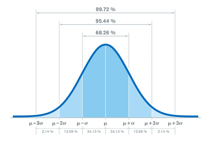
The assumption we can make about the data that follows a normal curve is that the area under the curve is relative to how many standard deviations we are away from the mean. The area between plus and minus one standard deviation from the mean contains 68% of the data. Two standard deviations contains 95% of the data and three standard deviations contains 99.8% of data.
Real-life example: Let’s say we want to create grab-and-go donut hole boxes in our local donut shop. We notice that customers buy 20 donut holes on average when they order them fresh from the counter and the standard deviation of the normal curve is 5. If we want to serve 95% of customers interested in donut holes, we should offer sizes two standard deviations away from the mean, on both sides of the mean. So, sizes of 10 (20-5-5), 15 (20-5), 20 (the average), 25 (20+5) and 30 (20+5+5).
How Does Standard Deviation Relate to Six Sigma?
First and foremost, it’s important to understand that a standard deviation is also known as sigma (or σ). And Six Sigma is a methodology in which the goal is to limit defects to six “sigmas,” three above the mean and three below the mean. Anything beyond those limits requires improvements. Because three standard deviations contains 99.8% of the data in a set, Six Sigma requires continuous refinement to consider improvements that fall within that 0.2% of data in the set.
Steps to Calculate Standard Deviation
Follow these two formulas for calculating standard deviation. The first formula is for calculating population data and the latter is if you’re calculating sample data.
The formula for standard deviation depends on whether you are analyzing population data, in which case it is called σ or estimating the population standard deviation from sample data, which is called s:
The steps to calculating the standard deviation are:
- Calculate the mean of the data set (x-bar or 1. μ)
- Subtract the mean from each value in the data set.
- Square the differences found in step 2
- Add up the squared differences found in step 3
- Divide the total from step 4 by either N (for population data) or (n – 1) for sample data (Note: At this point, you have the variance of the data)
- Take the square root of the result from step 5 to get the standard deviation.
Example:
Step 1: The average depth of this river, x-bar, is found to be 4’.
Step 5: The sample variance can now be calculated:
Step 6: To find the sample standard deviation, calculate the square root of the variance:

Why is Standard Deviation Important?
Standard deviation is important because it measures the dispersion of data – or, in practical terms, volatility. It indicates how far from the average the data spreads. This helps you determine the limitations and risks inherent in decisions based on that data.
Real-life example: When considering investing in a stock, you can use standard deviation to determine risk. A stock with an average price of $50 and a standard deviation of $10 can be assumed to close 95% of the time (two standard deviations) between $30 ($50-$10-$10) and $70 ($50+$10+$10). It’s safe to assume that 5% of the time, it will plummet or soar outside of this range. If you were to compare this to a stock that has an average price of $50 but a standard deviation of $1, then it can be assumed with 95% certainty that the stock will close between $48 and $52. The second stock is less risky, more stable. The higher the standard deviation in relation to the mean, the higher the risk. Blue-chip stocks, for example, would have a fairly low standard deviation in relation to the mean.
Standard deviation has many practical applications, but you must first understand what it’s telling you about the data. Additionally, standard deviation is essential to understanding the concept and parameters around the Six Sigma methodology.


